Large Model Training and Inference

1. Why AI Infra Matters

A minimal training loop only has a few steps: feed data into the model, run the forward pass, compute the loss, backpropagate, and update the parameters.

When the model is small, a single GPU can handle the entire workload. As the model grows, the problem gradually shifts from “can the algorithm train?” to “can the system support the training process?”

A training job depends on at least three kinds of resources:

• Compute: whether the GPUs provide enough compute for matrix operations;
• Storage: whether data, model weights, and checkpoints can be read and written fast enough;
• Network: whether GPUs and nodes can exchange data efficiently.

GPU Utilization

On a single GPU, training depends on much more than the compute cores themselves. Model parameters and intermediate tensors are usually stored in HBM (High Bandwidth Memory). Kernels read data from memory, perform computation, and write results back.

For a 7B model using FP16, the parameters alone require roughly:

$$7\times10^9\times2\text{ Byte}\approx14\text{ GB}$$

Training also needs gradients, optimizer states, activations, and temporary buffers. So “7B parameters take about 14 GB” only describes the model weights; it does not mean a 14 GB GPU can train a 7B model.

Data Supply

Training data usually goes through cleaning, deduplication, filtering, format conversion, tokenization, and finally the DataLoader before reaching the GPU.

If the GPU consumes data faster than the storage system can provide it, the GPU ends up waiting on I/O. The hardware has not become slower, but its effective utilization drops.

This is why training systems use techniques such as Prefetch, Cache, parallel DataLoader, Sharding, high-speed NVMe SSDs, and, at larger scale, distributed file systems and GPU Direct Storage.

All of them serve the same goal: keep the compute devices from sitting idle while waiting for data.

Checkpointing and Fault Tolerance

If a job only runs for ten minutes, restarting it after a crash is usually acceptable. When training lasts for days or weeks, node failures, network issues, and machine crashes become much more costly.

A Checkpoint is therefore more than a copy of the model weights. A recoverable training state often includes model parameters, optimizer states, the current step, random states, and the current data position.

Checkpointing answers “where can training resume from?” Fault Tolerance answers “how does the system keep going after something fails?” At large scale, both become infrastructure problems rather than a single torch.save() call inside a training script.

Resource Scheduling

Once a cluster runs many jobs at the same time, another layer of problems appears: which GPUs should be assigned to which job, when should jobs start, how should priorities be handled, and what happens when a node fails?

Systems such as Slurm, Kubernetes, Volcano, and Ray focus mainly on resources and scheduling. Megatron-LM and DeepSpeed focus more on how to organize training after the GPUs have been allocated. NCCL handles common GPU collective communication, while CUDA sits closer to the actual execution on each GPU.

They often appear in the same stack, but they operate at different layers.

---

2. Distributed Training

As models grow, two limits usually appear first: the model no longer fits on a single GPU, or it technically fits but trains too slowly.

Multi-GPU training is not as simple as adding more cards. Data, parameters, and computation all need to be repartitioned, which leads to Data Parallelism, Tensor Parallelism, and Pipeline Parallelism.

Data Parallelism

Data Parallelism (DP) is the most straightforward approach: each GPU keeps a full copy of the model, while different GPUs process different data.

GPU0: full model + Batch A
GPU1: full model + Batch B
GPU2: full model + Batch C
GPU3: full model + Batch D

Figure 1. Forward pass, loss computation, and backward pass in Data Parallelism. Source: Infrasys-AI/AIInfra · Data Parallelism.

After the forward and backward passes, each GPU has computed different gradients. Gradient Synchronization is needed so that every replica applies the same parameter update.

A typical operation is All-Reduce. If two GPUs produce gradients of 2 and 4, both can update with the averaged gradient 3.

DP is conceptually simple and scales training throughput well, but it does not solve the problem of an oversized model because every GPU still keeps a complete model copy.

If one model requires 200 GB of memory while each GPU has only 80 GB, adding more data-parallel GPUs does not make the model fit.

Tensor Parallelism

Once a full model no longer fits on a single GPU, the model itself has to be split.

Tensor Parallelism (TP) usually partitions a large matrix or operator across multiple GPUs. For a linear layer

$$Y=XW$$

the weight matrix can be split by columns:

$$W=[W_1,W_2]$$

Two GPUs then compute XW₁ and XW₂ separately before combining the outputs.

This is one of the core forms of parallelism used in Megatron-LM.

TP solves the problem of oversized operators, but the split introduces frequent cross-GPU exchange of intermediate tensors. The more a model depends on cross-device communication, the more important network bandwidth and topology become.

Pipeline Parallelism

Pipeline Parallelism (PP) takes a different approach: different GPUs hold different layers.

For example, a 40-layer Transformer can be divided into four stages:

GPU0: Layer 1 ~ 10
GPU1: Layer 11 ~ 20
GPU2: Layer 21 ~ 30
GPU3: Layer 31 ~ 40

A sample has to pass through these stages in order. If only one batch is used, GPU1 waits for GPU0, GPU2 waits for GPU1, and a large fraction of time is lost to idle periods.

The batch is therefore usually divided into multiple Micro-batches so that different stages can process different micro-batches at the same time.

Time →
GPU0  MB1 MB2 MB3 MB4
GPU1      MB1 MB2 MB3 MB4
GPU2          MB1 MB2 MB3 MB4
GPU3              MB1 MB2 MB3 MB4

Even then, idle regions remain at the beginning and end of the pipeline. These are known as the Pipeline Bubble. More Micro-batches, 1F1B scheduling, Interleaved Pipeline execution, and better stage partitioning all aim to reduce this idle time.

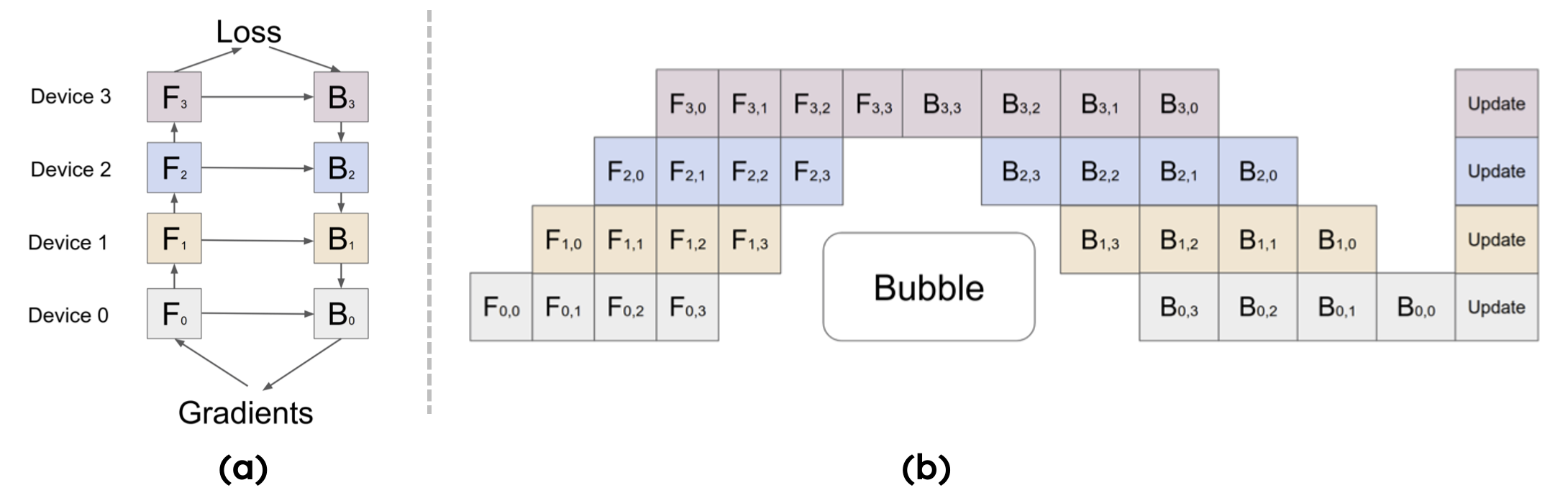
Figure 2. Micro-batch scheduling and pipeline bubbles in Pipeline Parallelism. Source: Infrasys-AI/AIInfra · Pipeline Parallelism.

3D Parallelism

Large-scale training rarely relies on only one parallelization strategy. DP, TP, and PP are often combined.

For example, 1024 GPUs can be organized as:

$$32\text{(DP)}\times8\text{(TP)}\times4\text{(PP)}=1024$$

This combination is commonly called 3D Parallelism.

A parallel strategy is not simply “more GPUs means more speed.” Every additional partition introduces new communication, synchronization, and load-balancing costs. Many AI Infra optimizations exist precisely to manage those costs.

---

3. Multi-GPU Communication

DP needs gradient synchronization, TP exchanges intermediate tensors, and MoE redistributes tokens across experts. Multi-GPU training always comes back to communication.

In the NVIDIA ecosystem, the standard communication library is NCCL (NVIDIA Collective Communications Library). Common collective operations include:

• All-Reduce: reduce data across GPUs and return the result to every GPU;
• All-Gather: each GPU holds one shard, and all GPUs gather the complete result;
• Reduce-Scatter: reduce first, then distribute different shards of the reduced result;
• All-to-All: each GPU sends different blocks to every other GPU, especially common in MoE.

Communication performance also depends on hardware topology. GPUs inside the same server may communicate through NVLink or similar high-speed interconnects, while cross-node communication relies more heavily on data-center networks such as InfiniBand or RoCE.

So “8 GPUs” only describes the quantity. Whether those GPUs span multiple nodes, how they are connected, and whether communication can overlap with computation all affect final throughput.

This is where Communication-Compute Overlap becomes useful: the GPU keeps computing one part while transferring data needed by the next, hiding as much communication latency as possible behind compute.

---

4. Memory Optimization

As parameter counts grow, GPU memory becomes one of the most direct constraints. But training memory cannot be estimated from model weights alone.

A training step roughly needs:

$$\text{Parameters}+\text{Gradients}+\text{Optimizer States}+\text{Activations}+\text{Buffers}$$

This explains a common situation: the weights fit in GPU memory, but training immediately runs out of memory.

ZeRO

In ordinary Data Parallelism, every GPU keeps a full copy of the model state. As the number of GPUs grows, a large amount of memory is spent on duplicated state.

ZeRO (Zero Redundancy Optimizer) reduces this redundancy.

ZeRO-1 shards Optimizer States. ZeRO-2 also shards Gradients. ZeRO-3 additionally shards Parameters.

             Parameters   Gradients   Optimizer States
ZeRO-1          full         full          sharded
ZeRO-2          full       sharded         sharded
ZeRO-3        sharded      sharded         sharded

Assume the model has Ψ parameters. FP16 parameters require 2Ψ bytes, FP16 gradients require another 2Ψ bytes, and optimizer-related states require KΨ bytes. Under conventional data parallelism, each GPU roughly stores:

$$(2+2+K)\Psi$$

If K=12, the total is 16Ψ. For a 7.5B-parameter model, these states take roughly 120 GB.

With N_d data-parallel GPUs, ZeRO-3 further shards these states. In an idealized form, each GPU stores approximately:

$$\frac{(2+2+K)\Psi}{N_d}$$

With 64 GPUs, 120 GB becomes about 1.875 GB per GPU.

This number only covers the model states sharded by ZeRO. Activations, temporary buffers, communication buffers, and other runtime memory still remain.

The trade-off in ZeRO-3 is direct: because parameters are no longer fully resident on each GPU, they must be fetched from other GPUs when needed. Lower memory usage usually means more communication.

This kind of Trade-off runs through most of AI Infra: a resource saved in one dimension often reappears as a cost somewhere else.

FSDP and ZeRO-3

PyTorch FSDP (Fully Sharded Data Parallel) also shards parameters, gradients, and optimizer states across multiple ranks, so it is often compared with ZeRO-3.

Their implementations and interfaces are not identical, but the main idea for learning purposes is the same: Data Parallelism does not necessarily mean every GPU permanently stores a complete copy of the model state.

Offload

Another approach is Offload. Parameters or optimizer states that are not immediately needed can be moved from GPU HBM to CPU RAM or even NVMe SSDs.

GPU HBM ↔ CPU RAM ↔ NVMe SSD

This increases available capacity, but access latency rises sharply, and data movement has to cross PCIe or the network.

Offload solves “can it fit?” but not necessarily “can it run fast?” If data cannot be moved back to the GPU in time, the saved memory simply turns into extra waiting.

Gradient Accumulation

Gradient Accumulation addresses a different memory constraint.

If only 8 samples fit in memory at once but an effective Batch Size of 32 is desired, four forward/backward passes can accumulate gradients before one parameter update.

$$8\times4=32$$

This reduces the amount of data that must fit in memory at once, but the computation is still performed, so gradient accumulation should not be mistaken for free speedup.

---

5. Single-GPU Performance

Solving OOM only means the program can run. The harder question in AI Infra is whether the GPU is actually being used efficiently.

One common metric is MFU (Model FLOPs Utilization). If the hardware can theoretically deliver 1000 TFLOPS but only about 400 TFLOPS are effectively used for model computation during training, MFU is roughly 40%.

A GPU may be underutilized for many reasons: waiting for data, waiting for communication, waiting for other GPUs, Pipeline Bubbles, kernels that are too small, slow memory access, load imbalance, or inefficient scheduling.

These seemingly different issues all point to the same question: is time being spent on useful computation, or on moving data and waiting?

Kernel Fusion

GPU operations are executed through Kernels. If a model operator is broken into many small kernels, each kernel launch adds overhead, and intermediate tensors may repeatedly be written to HBM and read back again.

For example, if LayerNorm, Dropout, and Add are executed separately, more intermediate memory traffic is created. Kernel Fusion combines multiple operations into fewer kernels, reducing launch overhead and memory traffic.

This highlights an important system-level fact: the same FLOPs do not necessarily imply the same runtime.

FlashAttention

Standard Attention is:

$$\mathrm{Attention}(Q,K,V)=\mathrm{softmax}\left(\frac{QK^T}{\sqrt d}\right)V$$

For sequence length N, the intermediate Attention Matrix scales with N². The problem with a conventional implementation is not only the matrix size, but also the repeated movement of intermediate results between HBM and on-chip memory.

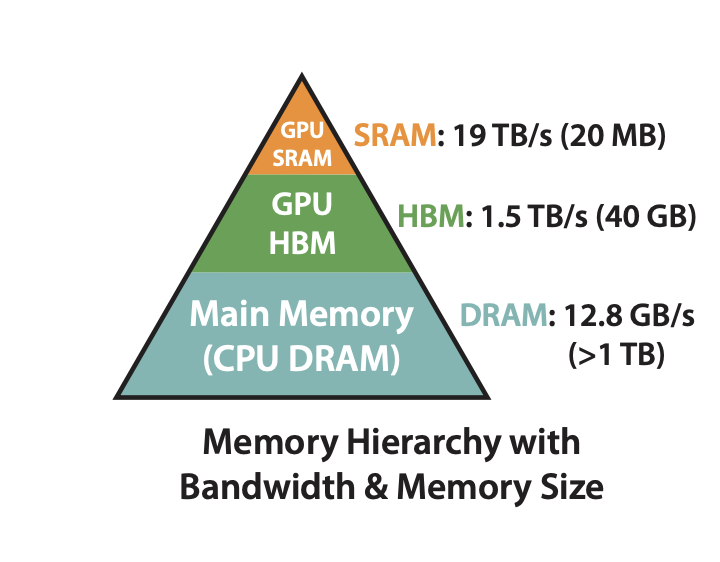
Figure 3. GPU Memory Hierarchy: larger memory is usually farther from the compute cores and offers lower bandwidth. Source: Infrasys-AI/AIInfra · Flash Attention. The values shown in the figure correspond to the A100 example used in the course.

FlashAttention does not change the mathematical definition of Attention. It reorganizes the computation so that, through Tiling, more intermediate work stays in on-chip SRAM / Shared Memory, reducing reads and writes to HBM.

This type of approach is usually described as an IO-Aware Algorithm.

FlashAttention is a useful example of how I think about AI Infra: the mathematical operation stays the same, but performance changes because the Memory Hierarchy is used differently. Many “system optimizations” are not external tools wrapped around a model; they reach directly into how operators are executed.

Mixed Precision

FP32 uses 4 bytes per value, while FP16 / BF16 usually use 2 bytes. Lower precision reduces memory usage and can also improve effective Tensor Core throughput.

But a smaller numerical range and lower precision also introduce Overflow, Underflow, and numerical instability. Training therefore does not simply convert every tensor to the same low-precision format.

AMP (Automatic Mixed Precision) chooses suitable precision based on the operator. In PyTorch, a common pattern is:

with torch.autocast(device_type="cuda"):
    output = model(x)

The real goal of low-precision training is not simply “smaller numbers,” but a balance among speed, memory, and stability.

Quantization

Quantization is more commonly used during inference, for example by converting FP16 weights to INT8 or INT4.

Reducing 16-bit values to 4-bit values cuts theoretical parameter storage to one quarter, ignoring quantization metadata and auxiliary scales.

PTQ (Post-Training Quantization) quantizes a model after training. QAT (Quantization-Aware Training) simulates quantization error during training so that the model can adapt to low-bit representations.

Quantization is another reminder that model performance is not determined only by parameter count. The numerical format used to store and compute those parameters is itself part of the infrastructure design space.

Hardware-Aware Optimization

The same algorithm may not have the same optimal implementation on different GPUs because Tensor Cores, memory bandwidth, cache behavior, instruction sets, and communication capabilities all differ.

Hardware-Aware Optimization focuses on how an algorithm maps onto specific hardware. Triton, CUTLASS, TensorRT-LLM, TVM, and XLA all relate to this problem, although they sit at different layers of the stack.

The Roofline Model, which often appears when learning CUDA, also belongs to this perspective: is a kernel limited more by compute throughput or by memory bandwidth?

---

MoE and Sparse Computation

A Dense Model usually sends every Token through the same main set of parameters. MoE (Mixture of Experts) introduces multiple Experts, and a Router selects only a small subset for each Token.

Token
  ↓
Router
  ↓
Expert 3 + Expert 7

This allows Total Parameters to be much larger than the Active Parameters used for each Token.

At first glance, this sounds like “more parameters without proportionally more computation,” but the system complexity increases substantially.

If a large fraction of Tokens are routed to Expert 1 while Expert 2 receives very little traffic, Load Imbalance appears. When Experts are spread across multiple GPUs, Tokens also need to be redistributed using All-to-All Communication.

A Router inside the model therefore affects Expert Placement, Expert Parallelism, communication topology, and load balancing.

MoE shows why the boundary between model algorithms and Infra is not fixed. Once the computation graph changes, the system has to reconsider where data lives, when it moves, and how to avoid turning some GPUs into hotspots.

---

6. Pre-training and Post-training

Large-model training does not end after a single pre-training run. Pre-training, SFT, and RLHF / DPO have different execution patterns and therefore place different demands on the system.

Pre-training

The goal of Pre-training is to learn general language patterns, knowledge, and some reasoning ability from large-scale data, producing a Base Model.

GPT-style models usually use CLM (Causal Language Modeling), predicting the next Token from all previous Tokens:

$$P(x_t\mid x_1,x_2,\dots,x_{t-1})$$

The full sequence can be written as:

$$P(x_1,x_2,\dots,x_T)=\prod_{t=1}^{T}P(x_t\mid x_{<t})$$

BERT-style models are more closely associated with MLM (Masked Language Modeling), where the model reconstructs masked positions from bidirectional context.

CLM and MLM describe training objectives. DP, TP, ZeRO, and FlashAttention describe how the training computation is executed. These ideas often appear together, but they belong to different dimensions.

SFT and LoRA

SFT (Supervised Fine-Tuning) uses input-target pairs to make a Base Model respond more consistently to task requirements.

For large models, full fine-tuning updates every parameter and brings high memory and storage costs. This led to PEFT (Parameter-Efficient Fine-Tuning).

LoRA (Low-Rank Adaptation) is one of the most common PEFT methods.

Assume the original weight is W. Instead of learning a full ΔW, LoRA parameterizes the update with low-rank matrices:

$$\Delta W=BA$$

where:

$$A\in\mathbb{R}^{r\times d},\qquad B\in\mathbb{R}^{d\times r},\qquad r\ll d$$

The updated weight becomes:

$$W'=W+BA$$

When d is large and r is small, the number of trainable parameters is far below that of a full weight matrix.

PEFT also includes Adapter, Prefix Tuning, and Prompt Tuning. Their common goal is not to make the model itself smaller, but to reduce how many parameters each fine-tuning task needs to update and store.

From an Infra perspective, this affects GPU Sharing, task scheduling, Memory Isolation, Checkpointing, and Job Queues: the same GPU pool can potentially support more fine-tuning jobs at once.

RLHF

RLHF (Reinforcement Learning from Human Feedback) is more complex than ordinary SFT.

A typical pipeline first collects human preferences, then trains a Reward Model, and finally optimizes a Policy using reinforcement learning. The system may involve a Policy Model, Reward Model, Reference Model, Rollout, Inference, and Training at the same time.

A single “training job” is no longer just one model running forward and backward passes. It becomes a data-generation, evaluation, and update pipeline involving multiple models.

DPO

DPO (Direct Preference Optimization) directly optimizes a model using preference pairs made of a Preferred Answer and a Rejected Answer.

Compared with classic RLHF, it can remove the need for a separate Reward Model and parts of the reinforcement-learning pipeline, making the engineering path shorter.

This does not mean DPO is simply a “lighter version of RLHF.” Their optimization formulations are different. From the Infra perspective, the more useful observation is that once the training algorithm changes, the required model count, sampling pattern, memory usage, and data flow change with it.

---

7. Model Evaluation and Evaluation Infra

After training, the question changes from “is the Loss going down?” to “did the model actually get better?”

Perplexity (PPL) measures predictive quality in language-modeling tasks. A common form is:

$$\mathrm{PPL}=\exp\left(-\frac{1}{N}\sum_{i=1}^{N}\log P(x_i\mid x_{<i})\right)$$

Under the common setting where Loss is the mean cross-entropy, it is also often written as:

$$\mathrm{PPL}=e^{\mathrm{Loss}}$$

Lower PPL means better prediction under the language-modeling objective, but it does not by itself measure chat quality, reasoning, safety, or tool use.

Modern LLM evaluation therefore relies on many Benchmarks:

• MMLU: broad academic knowledge and reasoning;
• GPQA: difficult scientific knowledge and reasoning;
• SWE-bench: asks a model to understand a repository, modify code, and pass tests;
• BLEU / ROUGE: still used for reference-based tasks such as translation and summarization;
• Human Evaluation, LLM-as-a-Judge, and Task-specific Metrics: used for more open-ended generation tasks.

When a model has many Checkpoints and each one needs to run a full benchmark suite, evaluation itself becomes a large consumer of GPU and storage resources.

Evaluation Infra therefore includes batch scheduling, result caching, benchmark management, logging, version tracking, and visualization.

It resembles CI/CD in software engineering: when the model or data changes, training and testing need to run automatically, results need to be tracked, and those results determine whether the next iteration should continue.

Data → Train → Evaluate → Deploy → Monitor
  ↑                                  ↓
  └──────────── Collect Data ────────┘

This is also part of MLOps / LLMOps.

---

8. Inference Infra

A model may only be trained a few times, but once deployed, the same model may serve millions of requests.

The bottlenecks in inference are therefore different from those in training. Training emphasizes large-scale parallelism, backward propagation, and model states. Serving focuses more on Latency, Throughput, concurrent requests, and cost per Token.

KV Cache

A Decoder-only LLM needs the Key / Value states of all previous Tokens when generating each new Token. To avoid recomputing historical K and V at every step, those intermediate states are stored in the KV Cache.

As the number of requests and context lengths grow, KV Cache usage grows as well. During inference, “the model weights fit in memory” does not mean “the system can serve many long-context requests at once.”

This makes KV Cache management one of the central problems in inference Infra.

PagedAttention

vLLM’s PagedAttention splits the KV Cache into fixed-size Blocks and manages them in a way similar to virtual-memory paging.

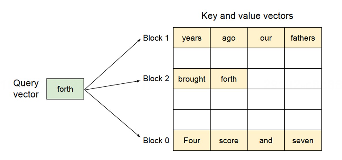
Figure 4. PagedAttention organizes the KV Cache in fixed-size blocks. Source: Infrasys-AI/AIInfra · Paged Attention; the original PagedAttention method is from Kwon et al., SOSP 2023.

This reduces fragmentation caused by large contiguous memory allocations and also makes it easier to share parts of the KV Cache across requests.

There is an important difference between this and FlashAttention. FlashAttention mainly optimizes data movement during Attention computation, while PagedAttention focuses on how the KV Cache is organized and allocated in Serving.

Both contain “Attention” in the name, but they solve different problems.

Continuous Batching

Traditional batches often enter and finish together. LLM requests, however, can have very different generation lengths: some end after a few dozen Tokens, while others continue for hundreds more.

If the whole batch is forced to finish together, completed requests keep occupying slots while waiting for the longer ones.

Continuous Batching allows completed requests to leave immediately and new requests to join the active batch, keeping GPU utilization higher over time.

Prefix Caching

Many requests may share the same System Prompt, long document prefix, or conversation history. Prefix Caching reuses the computation associated with those shared prefixes, reducing repeated Prefill work.

This turns “do requests share the same context?” into another systems optimization opportunity.

Speculative Decoding

One major limitation of autoregressive generation is that Tokens are produced sequentially. Speculative Decoding uses a smaller Draft Model to propose several candidate Tokens at once, which are then verified in parallel by the Target Model.

If the draft Tokens are accepted often enough, the number of serial Target Model steps can be reduced.

The main target here is the serial nature of the Decode path, not simply making the matrix multiplication for each Token faster.

Disaggregated Serving

Prefill and Decode do not have the same resource characteristics. Prefill is usually more compute-intensive, while Decode is often more sensitive to KV Cache and memory access.

Disaggregated Serving separates the two stages into different resource pools so that hardware configuration and scheduling can be optimized independently.

Common inference frameworks include vLLM, SGLang, TensorRT-LLM, and TGI. They are not direct substitutes in every sense, but all of them do significant work around Batching, KV Cache, Kernels, Parallelism, and Scheduling.

---

9. The AI Infra Stack

If these ideas are memorized only by name, they quickly fall apart again. Organizing them by the problem they solve is much more stable.

If the model is too large for a single GPU, TP, PP, ZeRO, FSDP, and Offload become relevant.

If many GPUs are available but scaling is poor, NCCL, communication topology, Pipeline Bubbles, Communication-Compute Overlap, and load balancing start to matter.

If theoretical GPU throughput is high but utilization is low, the focus shifts to Kernels, the Memory Hierarchy, Kernel Fusion, FlashAttention, the Roofline Model, and Hardware-Aware Optimization.

If the model uses MoE, the system must also deal with the Router, Expert Placement, Expert Parallelism, and All-to-All communication.

Once the model moves from training to deployment, the problems shift toward KV Cache, PagedAttention, Continuous Batching, Prefix Caching, Speculative Decoding, Quantization, and Disaggregated Serving.

AI Infra is therefore not one framework, and it is not just CUDA. It is a set of systems problems that run through the entire model lifecycle: how computation is partitioned, where data lives, when it moves, which devices communicate, and how limited resources are scheduled.

---

10. Learning Path

At this stage, it makes more sense to learn AI Infra in four layers rather than trying to study every framework at once.

Single GPU

Focus on:

• GPU architecture basics
• CUDA
• Memory Hierarchy
• Kernel
• Roofline Model
• Kernel Fusion
• FlashAttention

The goal is not to immediately write complex kernels from scratch, but to build an intuition for the relationship among computation, memory traffic, and parallelism.

Multi-GPU

Focus on:

• PyTorch DDP
• NCCL
• All-Reduce / All-Gather / Reduce-Scatter
• Tensor Parallel
• Pipeline Parallel
• ZeRO
• FSDP

By this stage, DP, TP, and PP should be more than definitions; it should be possible to explain what communication each strategy introduces.

Training Systems

Continue with:

• Megatron-LM
• DeepSpeed
• Checkpoint
• Fault Tolerance
• MoE
• Expert Parallelism
• Resource scheduling and training monitoring

This is where a single training script starts to be understood in the context of a real cluster.

Inference Systems

Focus on:

• KV Cache
• PagedAttention
• Continuous Batching
• Prefix Caching
• Speculative Decoding
• Quantization
• vLLM
• SGLang

This layer connects most directly to inference-engine work and also contains many small, measurable systems problems that are suitable for experiments.

---

11. Key Takeaways

1. The main thread of AI Infra is not a list of tools, but the constraints among Compute, Memory, Communication, Storage, and Scheduling.
2. DP splits data, TP partitions operators inside the model, and PP partitions layers; large-scale training often combines all three.
3. ZeRO / FSDP reduce duplicated model states through sharding, but lower memory usage usually comes with more communication.
4. GPU performance depends on more than FLOPs. Kernel Launch overhead, HBM traffic, and communication stalls can all become dominant bottlenecks.
5. FlashAttention is IO-Aware: the Attention math stays the same, but the data movement changes.
6. MoE introduces sparse activation but also brings routing, load balancing, and All-to-All communication into the system layer.
7. Training and inference have different bottlenecks. Inference especially depends on KV Cache, Batching, Latency, and Throughput.
8. Many AI Infra techniques are ultimately Trade-offs: there is rarely a free optimization among memory, compute, communication, latency, throughput, and cost.

---

12. References

1. ZOMI.
2. Rajbhandari, S. et al. ZeRO: Memory Optimizations Toward Training Trillion Parameter Models. SC 2020 / arXiv:1910.02054.
3. Shoeybi, M. et al. Megatron-LM: Training Multi-Billion Parameter Language Models Using Model Parallelism. arXiv:1909.08053.
4. Dao, T. et al. FlashAttention: Fast and Memory-Efficient Exact Attention with IO-Awareness. NeurIPS 2022 / arXiv:2205.14135.
5. Hu, E. J. et al. LoRA: Low-Rank Adaptation of Large Language Models. ICLR 2022 / arXiv:2106.09685.
6. Ouyang, L. et al. Training Language Models to Follow Instructions with Human Feedback. NeurIPS 2022 / arXiv:2203.02155.
7. Rafailov, R. et al. Direct Preference Optimization: Your Language Model is Secretly a Reward Model. NeurIPS 2023 / arXiv:2305.18290.
8. Kwon, W. et al. Efficient Memory Management for Large Language Model Serving with PagedAttention. SOSP 2023 / arXiv:2309.06180.

13. Copyright and Attribution

This article is a personal set of notes written while studying AI Infra. It is mainly based on the open-source Infrasys-AI/AIInfra course, with the material reorganized around the original papers and my own understanding. It does not represent official AIInfra documentation.

The course documentation and related materials in the AIInfra repository are distributed under the terms stated in its LICENSE, which uses the Apache License 2.0. The code is covered separately by LICENSE-CODE. Copyright for the original project belongs to ZOMI and the relevant contributors.

A small number of AIInfra course illustrations are used in this article, with the corresponding course page cited below each figure. The current Markdown file links directly to the images hosted by the course site and does not modify them. If an image in the original course comes from a paper, vendor document, or another third-party source, that original attribution should also be preserved rather than replaced by the AIInfra citation.

If this article is later deployed on a personal blog, it is better to store these images in the blog’s own static asset directory while keeping the figure captions and source links intact, so the article does not break if external image URLs change.