LLM Inference AI Infra

1. A Model That Runs Is Not Yet a Usable Service

Finishing training means the model can generate outputs. It does not mean the model is ready to serve real traffic.

Training usually cares more about final accuracy, total training time, and throughput under large batches. A training run may last for days or weeks, and the data is prepared in advance. Inference is different: requests arrive continuously, input and output lengths vary, and traffic changes over time.

A production inference system therefore has to balance several goals at once:

1. Latency: how long a single request takes;
2. Throughput: how many requests or tokens the system can process per unit time;
3. Concurrency: how many requests can be served at the same time;
4. Cost: how efficiently GPU resources are used;
5. Reliability: whether the service remains stable under traffic spikes or partial failures.

These goals often conflict. Larger batches can improve throughput, but waiting too long to form a batch increases queueing latency. Keeping preloaded model instances reduces cold-start delay, but idle instances increase cost.

That makes LLM inference a systems problem by nature:

$$\text{Inference Performance}=f(\text{Compute},\text{Memory},\text{Communication},\text{Scheduling},\text{Software Stack})$$

This is where AI infrastructure starts to diverge from model algorithms alone.

---

2. Inference Performance Metrics

Looking only at tokens/s can be misleading. An online service needs to distinguish overall throughput, time to the first token, and the speed of subsequent generation.

2.1 Latency and Throughput

Latency measures how long one request takes from entering the system to receiving a result.

Throughput measures how many requests or tokens the whole system can process in a given amount of time.

They are not the same objective. Some optimizations raise total throughput while making an individual request wait longer. Others reduce per-request latency but lower overall GPU utilization.

2.2 TTFT and TPOT

LLMs generate output token by token, so total latency can be split further.

TTFT, or Time To First Token, measures how long it takes from request arrival until the first output token is produced.

A rough decomposition is:

$$\text{TTFT} \approx \text{Queueing}+\text{Preprocess}+\text{Prefill}+\text{First Sampling}$$

TPOT, or Time Per Output Token, measures the average time required to generate each new token after generation has started.

TTFT is more sensitive to queueing and Prefill, while TPOT is more closely tied to Decode efficiency.

2.3 P99

Average latency hides the small fraction of requests that become unusually slow.

P99 latency means that roughly 99% of requests finish within that value. P95, P99, and P99.9 are commonly referred to as tail latency metrics.

For an online service, the worst user experience often comes from a small group of very slow requests during peak traffic rather than from the average request. This is why an SLA, or Service Level Agreement, usually considers both availability and tail latency.

---

3. The Execution Path of an LLM Request

A text request usually goes through a pipeline like this:

Text
 ↓
Tokenizer
 ↓
Token IDs
 ↓
Prefill
 ↓
Build KV Cache
 ↓
Decode: generate one token at a time
 ↓
Sampling
 ↓
Streaming

Multimodal models make the preprocessing stage more complex. Images may go through resize, normalization, and a vision encoder; audio may require resampling, feature extraction, and an audio encoder. After that, the main systems questions still come back to compute, memory, scheduling, and communication.

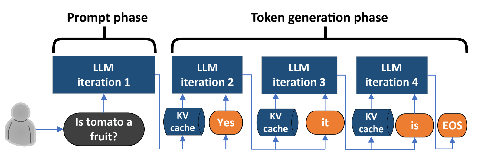
Source: ZOMI / AIInfra, “KV Cache Fundamentals”

The most important distinction in this figure is the input size and execution pattern of the two stages. Prefill processes the full prompt at once, computes K and V for those tokens, and builds the initial KV Cache. Decode then receives one new token at each step and reuses the cached K/V from previous tokens for attention.

Although both stages run the same Transformer, their workloads are different. Prefill naturally forms large matrix operations and offers high parallelism. Decode advances token by token; each step is smaller, but it repeatedly reads model weights and an increasingly large KV Cache. The later differences in TTFT, TPOT, Prefill-Decode disaggregation, and scheduling all begin here.

3.1 Input Preprocessing

Text must first be converted into token IDs by a Tokenizer before the model can process it.

This stage is usually much lighter than the Transformer itself. But as GPU execution becomes faster and request volume increases, CPU-side tokenization, image preprocessing, or audio feature extraction can become bottlenecks of their own.

Common optimizations include batching, multithreading, SIMD, caching repeated prompts, and distributing preprocessing work across CPUs, GPUs, or other accelerators.

3.2 Prefill

Prefill processes the entire input prompt and builds the KV Cache used by later generation steps.

A long prompt creates relatively large matrix operations, so Prefill usually has high parallelism. In many deployments it tends to be compute-bound: matrix multiplication and similar operations dominate more than memory movement does.

This is not an absolute rule. Prompt length, batch size, model architecture, and hardware can all move the bottleneck. Still, it explains why Prefill optimization often focuses on compute utilization.

3.3 Decode

After Prefill finishes, the model starts generating one token at a time.

Each new token requires reading the model weights and accessing the KV Cache built from previous tokens. The computation per step is smaller than in Prefill, but large amounts of data must be read repeatedly.

Decode therefore often becomes memory-bandwidth-bound.

The difference can be summarized as follows:

	Prefill	Decode
Input	Full prompt	One new token per step
Parallelism	High	Relatively low
Common bottleneck	Compute	Memory bandwidth
More directly affects	TTFT	TPOT

This difference continues to shape scheduling, hardware choices, and Prefill-Decode disaggregation later in the stack.

---

4. Four GPU Constraints That Matter for Inference

At least four hardware factors matter when judging whether a GPU is suitable for LLM inference:

1. compute capability;
2. memory capacity;
3. memory bandwidth;
4. communication between GPUs.

4.1 Compute

GPUs are the most common accelerators for LLM training and inference today, while NPUs and TPUs play similar roles on other platforms. Regardless of the hardware, much of a Transformer eventually reduces to large matrix operations such as:

$$Y=XW$$

Hardware specifications often report FLOPS, TFLOPS, PFLOPS, or TOPS.

FLOPS, Floating Point Operations Per Second, describes floating-point compute throughput. TOPS, Tera Operations Per Second, is also commonly used for lower-precision integer workloads such as INT8 and INT4.

Peak numbers at different precisions or for different operators are not directly comparable. An FP16 rating of 100 TFLOPS and an INT8 rating of 100 TOPS do not imply the same real LLM inference performance. Precision, Tensor Core support, kernel quality, and memory bandwidth all affect the final result.

4.2 Memory Capacity

GPU memory stores more than model weights.

Inference also needs space for the KV Cache, intermediate activations, and runtime buffers:

$$M_{GPU}=M_{weights}+M_{KV}+M_{activation}+M_{buffer}$$

For a 7B model, considering weights alone:

Precision	Bytes per parameter	Approx. 7B weight size
FP32	4 B	~28 GB
FP16 / BF16	2 B	~14 GB
INT8	1 B	~7 GB
INT4	0.5 B	~3.5 GB

Here, 7B means roughly seven billion parameters, not 7 GB.

Even if the weights fit in memory, high concurrency may still fail. Long-context requests can consume large amounts of additional space through the KV Cache.

4.3 Memory Bandwidth

Memory capacity determines how much data can fit. Memory bandwidth determines how fast that data can reach the compute units.

Decode repeatedly reads model weights and historical KV data. The GPU can therefore hit its memory-bandwidth limit before its arithmetic units are fully utilized.

A rough way to express the effective ceiling is:

$$\text{Actual Performance}\leq \min(\text{Compute Limit},\text{Memory Limit},\text{Communication Limit})$$

This is why moving to a GPU with much higher peak FLOPS does not necessarily increase Decode speed by the same proportion.

4.4 Multi-GPU Communication

Once a model no longer fits on one GPU, computation must be distributed across several devices.

Common interconnects include:

• PCIe: a general-purpose interconnect between CPUs, GPUs, and other devices;
• NVLink / NVSwitch: high-bandwidth interconnects for GPUs within a node;
• InfiniBand: a common high-speed network for multi-node training and inference clusters;
• RDMA, Remote Direct Memory Access: data transfer that minimizes CPU involvement across machines;
• RoCE, RDMA over Converged Ethernet: RDMA capabilities over Ethernet networks.

The more frequently a parallel strategy synchronizes across GPUs, the more likely communication is to enter the critical path. Fast local computation cannot compensate for slow synchronization between devices.

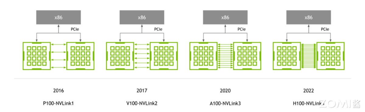
Source: ZOMI / AIInfra, “LLM Inference and AI Infrastructure”

With multiple GPUs, execution no longer happens only inside one device. Data exchange between GPUs becomes part of the execution path. Tensor Parallelism, for example, splits matrix computation within the same layer across multiple GPUs, so partial results must be synchronized frequently. Interconnect bandwidth and latency can therefore directly determine how long a layer takes to finish.

The point of this figure is not to memorize the exact NVLink topology. It is to see that the finer the model is partitioned, and the more often devices must synchronize, the more likely communication becomes a real bottleneck rather than a secondary overhead.

---

5. Storage Hierarchy and KV Cache

Not all data around a GPU lives in the same type of storage. Faster storage is usually smaller and more expensive.

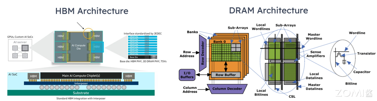
Source: ZOMI / AIInfra, “LLM Inference and AI Infrastructure”

This figure is easiest to read along one trend: speed decreases while capacity increases and cost per byte falls. HBM sits closest to the GPU and is best suited for weights and active KV Cache data that are accessed repeatedly. DRAM can hold offloaded weights or colder data. NVMe and object storage trade even more access speed for much larger capacity.

A deployment does not need to use all of these layers. The hierarchy mainly captures a data-placement rule: frequently accessed data on the critical path should stay as close to the GPU as possible. Once HBM becomes tight, the problem changes from simply “does it fit?” to “what deserves to stay in HBM, and what can be moved elsewhere?”

Faster / smaller capacity
        ↑
       HBM
        ↓
       DRAM
        ↓
       NVMe
        ↓
    Object Storage
        ↓
Slower / larger capacity

HBM, High Bandwidth Memory, usually stores current model weights, active KV Cache entries, and the activations needed by the current computation.

DRAM, Dynamic Random Access Memory, offers larger capacity and can hold offloaded weights, colder KV Cache data, or preprocessing results.

NVMe SSDs trade more latency for more capacity and are suitable for cold models, checkpoints, or infrequently accessed data.

Object stores such as S3, OSS, COS, and MinIO are better suited for long-term storage of model weights, datasets, logs, and archives.

The basic rule is simple: the more frequently data is accessed, the closer it should remain to the GPU.

5.1 How KV Cache Grows

During autoregressive generation, each historical token produces a Key and a Value. Later tokens still need those results. Recomputing them at every generation step would be expensive.

The previous K/V tensors are therefore stored in the KV Cache.

Its size can be expressed conceptually as:

$$M_{KV}\propto B\times S\times L\times N_{KV-head}\times D_{head}\times 2$$

where:

• B: batch size;
• S: sequence length;
• L: number of Transformer layers;
• N_KV-head: number of KV heads;
• D_head: dimension of each head;
• 2: both Key and Value must be stored.

Longer sequences and higher concurrency both increase KV Cache usage.

This explains a common deployment failure: the model weights fit comfortably on the GPU, but the service still runs out of memory under load. The remaining memory is often consumed by a growing KV Cache.

5.2 PagedAttention

A traditional KV Cache implementation that reserves large contiguous regions for each request can cause fragmentation and waste memory through over-allocation.

PagedAttention borrows the idea of paging from operating systems. It divides the logical KV Cache into blocks and maps them to physical GPU memory blocks:

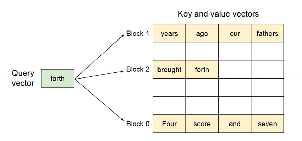
Source: ZOMI / AIInfra, “PagedAttention Fundamentals”

The key idea in this figure is that logical continuity and physical continuity are separated. A sequence still sees its KV Cache as ordered logical blocks. In physical GPU memory, however, those blocks may live in completely different locations, with a block table maintaining the mapping.

As the sequence grows, the system does not need to reserve one large contiguous region in advance. It can allocate another physical block only when the current one is nearly full. When the request finishes, those blocks can be returned immediately and reused by other requests. PagedAttention changes the memory-management strategy of the KV Cache; it does not change the mathematics of Attention itself.

Logical KV Blocks
       ↓
   Block Mapping
       ↓
Physical GPU Blocks

The goal is not to modify the Attention formula, but to make KV Cache allocation, reuse, and reclamation more flexible.

This became one of the defining ideas behind early versions of vLLM.

---

6. Inference Engines: Resource Management and Scheduling

The model itself sits above several software layers before work finally reaches the GPU:

Model
  ↓
Inference Engine
  ↓
Compiler / Graph Optimization
  ↓
Operator Library
  ↓
GPU Kernel
  ↓
GPU

The upper layers describe what computation is needed. Moving downward, the system becomes increasingly concerned with how that computation is mapped efficiently onto the GPU.

6.1 cuBLAS / CUTLASS

cuBLAS is NVIDIA’s high-performance linear algebra library. Many linear layers in Transformers eventually reduce to GEMM, or General Matrix Multiplication, and cuBLAS provides mature optimized implementations for those operations.

It is often the right choice when a strong general-purpose implementation is enough.

CUTLASS is also an NVIDIA CUDA linear algebra library, but it exposes much more control. Tile sizes, thread blocks, data layouts, precision, and Tensor Core usage can all be customized.

The difference is not that one is simply “fast” and the other “slow.” The difference is the level of control: cuBLAS provides mature general implementations, while CUTLASS is useful when kernel structure itself needs to be tuned.

6.2 vLLM

vLLM focuses on resource management and scheduling for high-throughput LLM serving, including:

• KV Cache management;
• PagedAttention;
• Continuous Batching;
• multi-request scheduling.

Its main concern is not how to implement a single matrix multiplication. It is how requests with very different lengths can share GPU resources efficiently.

6.3 SGLang

SGLang also targets efficient inference, but extends the runtime to structured generation, prompt reuse, agent and tool calling, and multi-stage generation programs.

The goal is no longer just to execute one model call efficiently. It is to let more complex generation programs reuse prefixes, caches, and computation as well.

6.4 TensorRT-LLM

TensorRT-LLM sits closer to hardware-specific optimization on NVIDIA GPUs, including quantization, kernel optimization, multi-GPU execution, and implementations tuned for specific hardware characteristics.

vLLM makes request scheduling and KV Cache management especially visible. TensorRT-LLM makes it easier to see how far down the stack software can go when the goal is to extract maximum performance from NVIDIA GPUs.

---

7. Batching and Throughput

GPUs are designed to execute many operations in parallel. Running requests one by one can leave a large fraction of the hardware idle, so inference systems group multiple requests into a batch.

Increasing batch size often improves throughput:

$$\text{Batch Size}\uparrow \Rightarrow \text{Throughput}\uparrow$$

But waiting too long to form a batch increases queueing latency.

Batching in online inference is therefore not about making the batch as large as possible. It is a dynamic trade-off between latency and throughput.

7.1 Continuous Batching

Static batches work poorly when requests generate outputs of different lengths.

[A B C]
A has finished, but the batch is still waiting for B and C

Continuous Batching lets completed requests leave immediately and fills the newly available slots with new requests:

Time 1: [A B C]
A finishes

Time 2: [D B C]
B finishes

Time 3: [D E C]

The GPU no longer has to wait for an entire batch to finish before accepting more work, which improves utilization in online serving.

PagedAttention makes KV Cache placement more flexible. Continuous Batching makes request admission and removal more flexible. Both aim to reduce GPU time and memory that would otherwise be wasted.

---

8. Prefill-Decode Disaggregation

Prefill tends to be compute-intensive, while Decode depends more heavily on memory bandwidth and sequential token generation.

If both workloads share the same pool of GPUs, they compete for resources and make scheduling less predictable.

Prefill-Decode Disaggregation, often shortened to PD disaggregation, places the two stages on different resources:

Request
  ↓
Prefill GPU
  ↓
KV Cache Transfer
  ↓
Decode GPU
  ↓
Output

This allows Prefill and Decode to use hardware and autoscaling policies that better match their workloads, while also reducing interference between them.

The cost is that the KV Cache must be transferred from the Prefill side to the Decode side.

PD disaggregation is therefore not automatically faster. It makes sense only when:

$$\text{Resource Isolation Benefit} > \text{KV Transfer Cost}$$

That pushes the problem back toward high-speed interconnects such as NVLink, InfiniBand, RoCE, and RDMA.

A design that initially looks like an inference-engine scheduling decision can end up depending on networking and hardware. This kind of cross-layer coupling is typical in AI infrastructure.

---

9. Kernels and Data Movement

Two implementations can use the same model equations and still run at very different speeds because the GPU ultimately executes low-level kernels.

9.1 The GPU Memory Hierarchy

Data inside a GPU moves through several levels of storage:

HBM / Global Memory
        ↓
Shared Memory
        ↓
Register
        ↓
CUDA Core / Tensor Core

HBM has large capacity but sits farther from the compute units. Shared Memory is faster and is shared by threads within the same thread block. Registers are closest to the compute units, but their capacity is extremely limited.

Many GPU optimizations reduce to the same basic idea: avoid repeatedly fetching the same data from HBM, and reuse data as much as possible once it has been moved into faster on-chip storage.

9.2 Operator Fusion

When several small operators run one after another, intermediate results may be written back to HBM and then loaded again by the next kernel:

A
↓ write to HBM
B
↓ write to HBM again
C

Operator Fusion combines several operations into a single fused kernel:

A + B + C
    ↓
Fused Kernel

The main gains come from reducing kernel launches and reducing memory traffic for intermediate data.

Fusion is not always better when taken further. A very large kernel may consume too many registers or too much Shared Memory, reducing occupancy and parallelism.

9.3 Kernel Tuning

GPU kernel efficiency depends on thread organization, tile size, Shared Memory usage, register usage, memory alignment, and related details.

A common NVIDIA GPU execution hierarchy includes:

• Thread: the basic execution unit;
• Warp: typically a group of 32 threads;
• Block: a group of threads that can share Shared Memory;
• Grid: all blocks launched by one kernel invocation.

Kernel tuning is not about maximizing one resource in isolation. It is about balancing parallelism, register pressure, Shared Memory usage, and compute-unit utilization.

For example, giving each thread more registers may make the thread itself more comfortable, but it can reduce the number of threads that can reside on the GPU at the same time.

9.4 FlashAttention

Standard Attention can be written as:

$$\text{Attention}(Q,K,V)=\text{Softmax}\left(\frac{QK^T}{\sqrt d}\right)V$$

FlashAttention does not change this formula. It changes how data moves between HBM and on-chip memory.

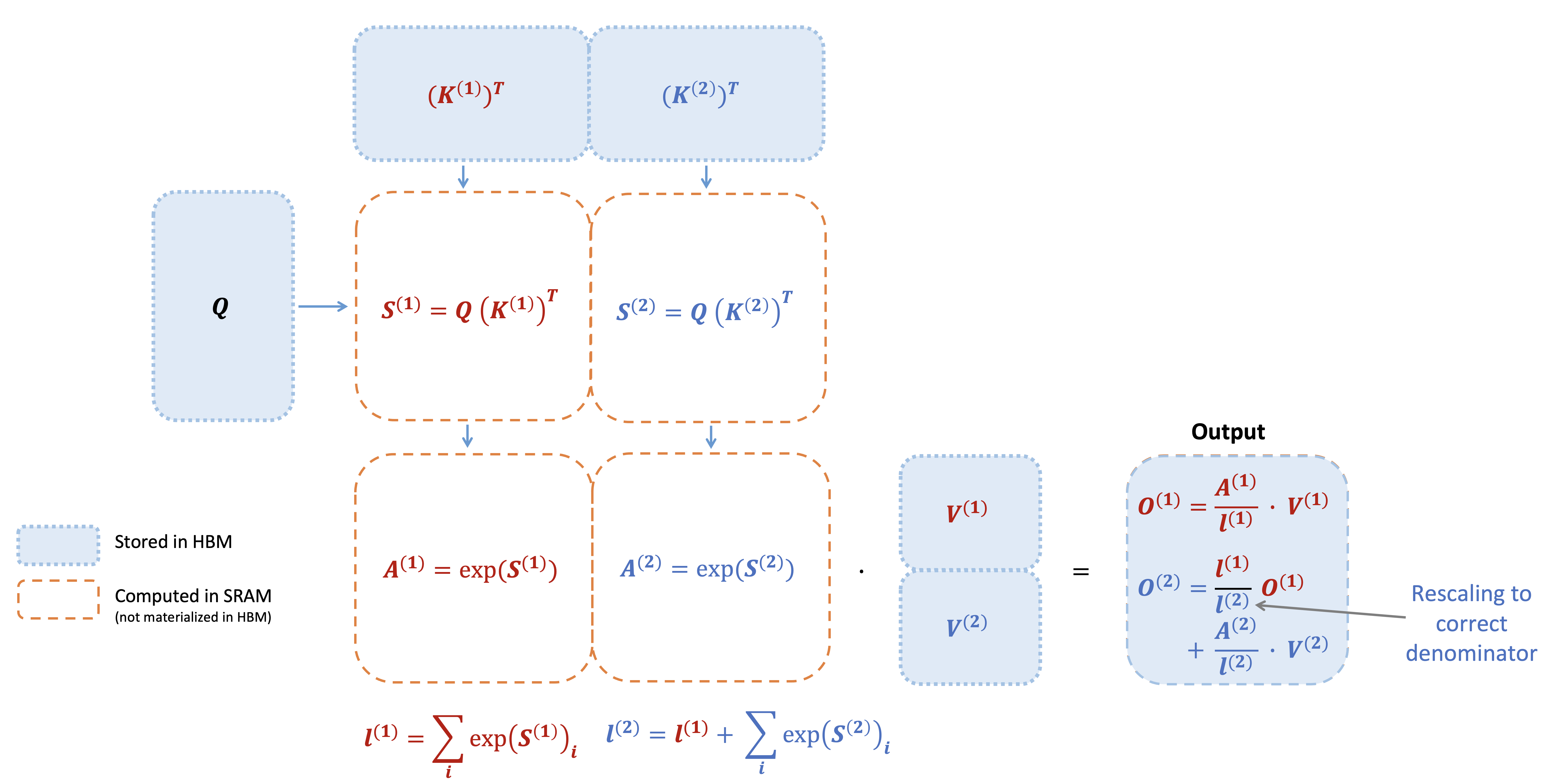
Source: Tri Dao, FlashAttention Recap

In the figure, the blue blocks represent data stored in HBM, while the orange dashed region represents local computation performed in faster on-chip SRAM. FlashAttention loads K and V in tiles and processes only part of the attention computation at a time, instead of first materializing the full QKᵀ matrix and writing it back to HBM.

The variables l and O on the right track the Softmax normalization state and partial outputs accumulated across tiles. When another K/V tile is loaded, the existing result is rescaled under the updated normalization and then merged with the new tile’s contribution. The final result is still equivalent to standard Attention; only the order of computation and where intermediate data lives have changed.

That is the core optimization behind FlashAttention: tiling and careful reorganization of intermediate results reduce data movement between HBM and on-chip SRAM. This is why FlashAttention is described as an I/O-aware algorithm. Here, I/O refers to data movement across the GPU memory hierarchy rather than disk or user input/output.

---

10. Model Compression

The first hard limit in inference is often that the model does not fit. The second is that it does not run fast enough.

Some techniques therefore reduce the resource footprint of a single model, while others distribute the model across more GPUs.

10.1 Quantization

Quantization uses fewer bits to represent model weights or activations.

A common precision path is:

FP32 → FP16 / BF16 → FP8 → INT8 → INT4

Moving weights from FP32 to INT8 can theoretically reduce their size to one quarter.

A fourfold reduction in weight size does not mean inference becomes four times faster. The real speedup depends on hardware support for the lower precision, kernel quality, dequantization overhead, and whether the workload is compute-bound or memory-bound.

Quantization is especially attractive during Decode because smaller weights reduce both memory-capacity pressure and memory-bandwidth demand.

10.2 Mixed Precision

Mixed Precision does not require every part of the model to use the same numerical format.

Numerically sensitive components can keep higher precision, while other parts use FP8, INT8, or INT4. The goal is to balance model quality, speed, and memory use.

10.3 Knowledge Distillation

Knowledge Distillation trains a smaller student model to learn from the output distribution, intermediate features, or generated outputs of a larger teacher model.

This is not simply a way to make an existing large model use less memory. It replaces the deployed model with a smaller one, reducing serving cost at the model level.

10.4 Pruning

Pruning reduces computation by removing unimportant parameters or structures.

Unstructured pruning produces sparse but irregular weights. GPUs may not gain an equivalent amount of real speed from that sparsity.

Structured pruning removes entire attention heads, channels, FFN units, or Transformer layers. The resulting structure remains regular and is therefore easier to map to real hardware acceleration.

---

11. Multi-GPU Parallelism

Multi-GPU inference usually addresses one of two problems: there are too many requests, or the model is too large. Data Parallelism is commonly used to scale service capacity, while models that do not fit on one GPU require Model Parallelism, which includes strategies such as TP, PP, and EP.

11.1 Data Parallelism

DP, Data Parallelism, replicates the full model across GPUs and assigns different requests to different replicas.

GPU0: full model → Request A
GPU1: full model → Request B
GPU2: full model → Request C

It is well suited for increasing total throughput and concurrency, but it cannot solve the problem of a single model being too large for one GPU.

11.2 Tensor Parallelism

TP, Tensor Parallelism, splits matrix computation inside the same layer across multiple GPUs.

        X
      /   \
   GPU0   GPU1
    W0     W1
      \   /
      Merge

Because multiple GPUs cooperate within the same layer, communication is frequent. High-speed links such as NVLink and NVSwitch can therefore have a direct impact on real performance.

11.3 Pipeline Parallelism

PP, Pipeline Parallelism, splits the model by layer ranges:

GPU0: Layers 1-10
  ↓
GPU1: Layers 11-20
  ↓
GPU2: Layers 21-30

Different pipeline stages can spend time waiting for one another, creating a pipeline bubble. Micro-batches can improve overlap, but they also make scheduling more complex.

11.4 Expert Parallelism and MoE

EP, Expert Parallelism, is mainly used for MoE, Mixture of Experts, models.

Instead of sending every token through every expert, a router selects only a small number of experts for each token:

Token
 ↓
Router
 ↓
Top-K Experts
 ↓
Selected Experts

This allows the total parameter count to be very large while keeping the number of parameters activated by each token relatively small.

If experts are distributed across different GPUs, tokens must be sent to the corresponding devices. EP therefore introduces substantial All-to-All communication.

Load imbalance is another problem. If many tokens are routed to the same expert, the system still has to wait for that expert even when other GPUs are idle.

MoE serving therefore introduces additional systems problems such as load-aware routing, expert capacity, expert replication, and dynamic scaling.

11.5 Long-Context Parallelism

With very long contexts, one GPU may not have enough memory for the full attention workload and KV Cache.

Sequence Parallelism, Context Parallelism, Ring Attention, Ulysses, and related techniques partition work along the sequence or context dimension.

The difficulty is that Attention creates dependencies across tokens. After the sequence is partitioned, K/V data or intermediate results still have to be exchanged across GPUs.

Long-context parallelism therefore balances two opposing goals: split the sequence far enough to fit, but not so aggressively that communication cost consumes the benefit.

---

12. Sampling and Streaming

12.1 Sampling

At each generation step, the model produces logits over the vocabulary. A sampling strategy then decides which token to generate next.

Common strategies include:

• Greedy Decoding: always choose the token with the highest probability;
• Top-K Sampling: keep only the K most probable candidates before sampling;
• Top-p / Nucleus Sampling: keep the smallest candidate set whose cumulative probability reaches p;
• Beam Search: maintain multiple candidate sequences at once, at the cost of additional compute and KV Cache usage.

Chat-oriented LLMs more commonly use combinations of Temperature, Top-p, and Top-k than large-scale Beam Search.

12.2 Streaming

Non-streaming generation waits until the full response is ready and then returns it all at once. Streaming starts sending tokens as soon as they are generated.

Token 1 → return
Token 2 → return
Token 3 → return

Streaming does not necessarily improve the model’s actual token generation rate, but it can substantially improve perceived latency.

Common protocols include SSE, Server-Sent Events, and WebSocket. SSE is widely used when the server only needs to push generated text continuously in one direction.

---

13. From Inference Engine to Online Service

An inference engine answers the question, “How can this batch of model requests run efficiently on the GPU?” A production service must also handle routing, autoscaling, failure recovery, and version management.

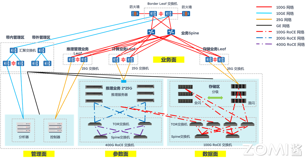
Source: ZOMI / AIInfra, “LLM Inference and AI Infrastructure”

At this layer, the focus expands from “how does one model run fast on a GPU?” to “how do many model instances provide a stable service over time?” GPUs and inference engines are still at the bottom of the stack, but they now sit behind instance management, request routing, load balancing, autoscaling, monitoring, and failure recovery.

Systems such as KServe and Ray Serve are therefore not replacements for vLLM or SGLang. They solve a different layer of the problem. The inference engine decides how a batch of requests should use the GPU efficiently; the serving layer decides which instance should receive a request, when more instances should be created, and what happens when an instance fails.

A typical serving path looks like this:

Client
  ↓
API Gateway
  ↓
Router / Load Balancer
  ↓
Model Instance
  ↓
vLLM / SGLang / TensorRT-LLM
  ↓
GPU

Kubernetes, KServe, Ray Serve, and similar systems often sit around this path to manage instance lifecycles and distributed orchestration.

13.1 Warm Pool

A model instance is not ready immediately after the process starts. It still needs to load weights, initialize the GPU, and build the runtime environment.

Starting from zero only after traffic rises can introduce a noticeable cold start.

A Warm Pool keeps some model instances preloaded and ready, trading idle resources for lower scale-out latency.

This optimization is not free: the more warm instances are kept around, the more unused resources may accumulate.

13.2 Autoscaling

Autoscaling increases or decreases the number of model instances according to traffic and resource state.

Reactive autoscaling adds capacity after load is detected. Predictive autoscaling tries to provision resources before the traffic peak arrives.

LLM instances are slower to start and load than ordinary stateless web services, making predictive scaling more valuable but also harder to get right.

13.3 Request Routing

Traditional services can route requests using strategies such as Round Robin, Least Connections, Geo Routing, or Version Routing.

LLM requests vary much more in cost. Two requests may both count as “one request,” while one contains only a few dozen prompt tokens and the other carries tens of thousands of tokens of context.

A better router may therefore consider:

• number of prompt tokens;
• predicted output length;
• KV Cache usage;
• GPU utilization;
• current queue length;
• Prefill / Decode load.

This is why LLM serving cannot simply copy load-balancing strategies from ordinary web services.

13.4 KServe / Triton / Ray

KServe is closer to Kubernetes-native model serving and focuses on deployment, autoscaling, routing, and model-version lifecycles.

Triton Inference Server is NVIDIA’s inference server. It provides HTTP and gRPC interfaces, dynamic batching, multi-model management, backend integration, and performance metrics.

It is not the same project as the Triton language used to write GPU kernels. The names are similar, but they live at very different levels of the stack.

Ray / Ray Serve is well suited to distributed tasks and multi-stage AI workflows, especially when models, agents, and tools form complex execution graphs that need to be scheduled across nodes.

---

14. The Full Inference Stack

From top to bottom, an LLM serving stack can be viewed roughly as:

┌────────────────────────────────────┐
│ Client / API                       │
├────────────────────────────────────┤
│ Routing / SLA / Load Balancing     │
├────────────────────────────────────┤
│ KServe / Ray Serve                 │
├────────────────────────────────────┤
│ vLLM / SGLang / TensorRT-LLM      │
├────────────────────────────────────┤
│ Batching / KV Cache / TP / PP / EP│
├────────────────────────────────────┤
│ Compiler / Fusion / Triton Kernel  │
├────────────────────────────────────┤
│ cuBLAS / CUTLASS / CUDA Kernel     │
├────────────────────────────────────┤
│ GPU / HBM / NVLink / RDMA          │
└────────────────────────────────────┘

When first learning these terms, it is easy to treat them as a flat list of unrelated technologies. Once connected into one stack, they are easier to understand as solutions to bottlenecks at different layers.

If the model does not fit, the discussion moves toward quantization, TP, PP, EP, and KV Cache management. If the model is too slow, the focus shifts to kernels, FlashAttention, fusion, and bandwidth. Once request volume grows, Continuous Batching, routing, autoscaling, and SLA become part of the problem.

A useful habit in inference optimization is therefore not to add every new technique to the system, but to identify the layer where the bottleneck actually sits.

Low GPU utilization does not automatically mean the GPU is too weak. High TTFT does not automatically mean Decode is slow. An OOM does not always mean the model weights are too large; the KV Cache may simply have consumed the remaining memory.

That is the most useful way I currently think about AI infrastructure: not as a collection of tool names, but as systems engineering driven by bottlenecks across the stack.

---

15. Key Takeaways

1. LLM inference is not about making one forward pass as fast as possible. It is about balancing latency, throughput, concurrency, cost, and reliability under limited resources.
2. Prefill and Decode have different workload characteristics. Prefill tends to be more compute-intensive, while Decode is more sensitive to memory bandwidth and KV Cache behavior.
3. KV Cache is a central resource in online inference. Longer contexts and higher concurrency increase its footprint, while PagedAttention improves how that memory is managed.
4. Inference engines are largely about scheduling and resource management. Systems such as vLLM and SGLang decide how requests are batched, how KV Cache is placed, and how resources are reused.
5. Many GPU optimizations are fundamentally about moving less data. Operator Fusion, tiling, and FlashAttention are all tightly connected to the cost of HBM access.
6. Communication enters the critical path once multiple GPUs are involved. TP, EP, long-context parallelism, and PD disaggregation can all lose their benefit if communication becomes too expensive.
7. Serving pushes the problem beyond the GPU. Routing, autoscaling, Warm Pools, and SLAs determine whether a model can serve real traffic reliably over time.
8. Locate the bottleneck before optimizing. Compute, memory capacity, bandwidth, communication, and scheduling can all be limiting factors, and stronger hardware alone does not guarantee a solution.

---

References

1. ZOMI / Infrasys-AI, AIInfra — 05. LLM Inference and AI Infrastructure
   https://github.com/Infrasys-AI/AIInfra/blob/main/00Summary/05InferStack.md

2. ZOMI / Infrasys-AI, AIInfra
   https://github.com/Infrasys-AI/AIInfra

3. Kwon et al., Efficient Memory Management for Large Language Model Serving with PagedAttention, SOSP 2023.
   https://arxiv.org/abs/2309.06180

4. Kwon et al., vLLM: Easy, Fast, and Cheap LLM Serving with PagedAttention, vLLM Official Blog.
   https://vllm.ai/blog/2023-06-20-vllm

5. Dao et al., FlashAttention: Fast and Memory-Efficient Exact Attention with IO-Awareness, NeurIPS 2022.
   https://arxiv.org/abs/2205.14135

6. Tri Dao, FlashAttention-3: Fast and Accurate Attention with Asynchrony and Low-precision, official blog (FlashAttention Recap figure).
   https://tridao.me/blog/2024/flash3/

7. Zheng et al., SGLang: Efficient Execution of Structured Language Model Programs.
   https://arxiv.org/abs/2312.07104

8. NVIDIA, TensorRT-LLM Documentation
   https://nvidia.github.io/TensorRT-LLM/

9. KServe Documentation
   https://kserve.github.io/website/

10. Ray Serve Documentation
    https://docs.ray.io/en/latest/serve/